


Fundamentals of Digital Measurement
In our previous discussion on power semiconductors, we highlighted the importance of precise numerical measurement for performance improvement. This requirement extends beyond semiconductors; digital measurement technology has become a cornerstone of modern industry, particularly with the rise of the IoT (Internet of Things).
Since the 1950s, the industry has shifted from analog to digital instrumentation. Traditional analog meters, familiar from basic educational settings, require users to visually estimate values between scale markings. While sufficient for simple checks, this method lacks the precision required for modern semiconductor design and performance evaluation.
Consequently, digital measuring instruments--which digitize data via A/D conversion--have become the standard in development environments. Today, a vast array of parameters, including voltage, current, temperature, and pressure, are captured and processed digitally.
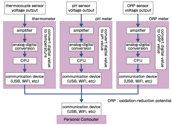
As pictured in the figure, the analog value acquired by each sensor is output as a voltage. After that, the signal (voltage) is amplified by an amplifier and A/D converted and then taken into a computer. The above figure gives an example of a sensor that is output as voltage. Image sensors used in Programmable Logic Controller (PLC) and digital cameras etc. A/D converts the (integrated) current value as the input value.
Recently, communication between sensors and computers, in some cases, tablets and smartphones, has often been performed via USB or wireless. Because it is difficult to lay cables for communication in the case of outdoor installation type sensors, such as digital instrument screens, especially, uploading of data by wireless is the mainstream. There are also cases where data is uploaded directly to the system built on the Internet.
Advancements in SoC (System on a Chip) technology have dramatically reduced the size and power consumption of computing modules. High-performance wireless communication chips are now available at a very low cost. This affordability allows for the deployment of sensor nodes in locations where cable installation is difficult, enabling data collection via wireless networks or direct cloud uploads.
With the establishment of LPWA (Low Power Wide Area) standards such as SIGFOX and LoRa, as well as 4G/5G cellular networks, it is now feasible to monitor hundreds of data points--such as temperature and humidity--with minimal power consumption. This collected "Big Data" is essential for applications ranging from infrastructure monitoring to agricultural automation.
The collected data is treated as big data, and the information processing according to the field such as social infrastructure monitoring, disaster prevention, and labor-saving of agriculture is performed and applied. IoT has been attracting attention in recent years as the use of such data has progressed.
Now, let's look at the change in the data value until such data is passed from the sensor to the computer. Here, the pH sensor is taken as an example.
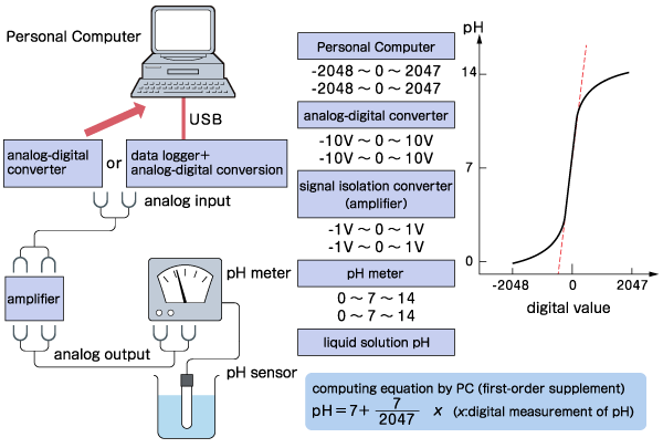
The value measured by the pH sensor converts a value between 0 and 14 when passed to the pH meter. The values at this time are still in analog form. There, it is once converted to a voltage in the range of -1 V to 1 V and sent to a signal isolation converter (amplifier). In the amplifier, it is amplified to -10V to 10V as the analog value. Then, A/D conversion is performed. As a result, the analog value of -10 V to 10 V is converted to a digital value of -2048 to 2047, which may be larger if it is a Power of 2, and then sent to a computer. Of course, you may convert it back to a digital value of 0-14 again before sending it to a computer. In any case, analog values are converted to voltages and then converted to digital values.
If the input is current, for example, in the programmable logic controller (PLC), the input value is often set to 0 to 20 mA of direct current, and this is often used by A/D conversion.
Measurement Resolution
When converting analog signals to digital values, "resolution" is a critical factor. Digital systems process information in binary (0 or 1), meaning resolution is expressed as a power of 2. For example, a 12-bit resolution provides 212 or 4096 discrete steps.
In a signed 12-bit system, this range is typically represented from -2048 to +2047. A higher bit count means the analog signal (e.g., -10 V to +10 V) is divided into finer steps, resulting in more precise measurements.
The table below illustrates the relationship between bit depth, integer range, and voltage resolution (LSB) for a 10 V full-scale range.
| bit | Range in decimal notation | |||||
|---|---|---|---|---|---|---|
| Signed | Unsigned | Resolution | Voltage value per stage (for 10VFS) |
%FS | dBFS | |
| 2 | -2 to 1 | 0 to 3 | 4 | 2.5V | 25 | -12 |
| 3 | -4 to 3 | 0 to 7 | 8 | 1.25V | 12.5 | -18 |
| 4 | -8 to 7 | 0 to 15 | 16 | 0.625V(625mV) | 6.25 | -24 |
| 5 | -16 to 15 | 0 to 31 | 32 | 0.313V(625mV) | 3.12 | -30 |
| 6 | -32 to 31 | 0 to 63 | 64 | 0.156V(156mV) | 1.56 | -36 |
| 7 | -64 to 63 | 0 to 127 | 128 | 0.0781V(78.1mV) | 0.78 | -42 |
| 8 | -128 to 127 | 0 to 255 | 256 | 0.0391V(39.1mV) | 0.39 | -48 |
| 9 | -256 to 255 | 0 to 511 | 512 | 0.020V(20mV) | 0.2 | -54 |
| 10 | -512 to 511 | 0 to 1023 | 1024 | 0.00977V(9.77mV) | 0.098 | -60 |
| 11 | -1024 to 1023 | 0 to 2047 | 2048 | 0.00488V(4.88mv) | 0.049 | -66 |
| 12 | -2048 to 2047 | 0 to 4095 | 4096 | 0.00244V(2.44mV) | 0.024 | -72 |
| 13 | -4096 to 4095 | 0 to 8191 | 8192 | 0.00122V(1.22mV) | 0.012 | -78 |
| 14 | -8192 to 8191 | 0 to 16383 | 16384 | 0.000610V(610μV) | 0.0061 | -84 |
| 15 | -16384 to 16383 | 0 to 32767 | 32768 | 0.000305V(305μV) | 0.003 | -90 |
| 16 | -32768 to 32767 | 0 to 65535 | 65536 | 0.000153V(153μV) | 0.0015 | -96 |
| 17 | -65536 to 65535 | 0 to 131072 | 131071 | 0.000076V(76μV) | 0.0008 | -102 |
| 18 | -131072 to 131071 | 0 to 262143 | 262144 | 0.000038V(38μV) | 0.0004 | -108 |
| 19 | -262144 to 262143 | 0 to 524287 | 524288 | 0.000019V(19μV) | 0.0002 | -114 |
| 20 | -524288 to 524287 | 0 to 1048575 | 1048576 | 0.00000954V(9.54μV) | 0.0001 | -120 |
| 21 | -1048576 to 1048575 | 0 to 2097151 | 2097152 | 0.00000476V(4.76μV) | 0.000048 | -126 |
| 22 | -2097152 to 2097151 | 0 to 4194303 | 4194304 | 0.00000238V(2.38μV) | 0.000024 | -132 |
| 23 | -4194304 to 4194303 | 0 to 8388607 | 8388608 | 0.00000119V(1.19μV) | 0.000012 | -138 |
| 24 | -8388608 to 8388607 | 0 to 16777215 | 16777216 | 0.000000596V(596nV) | 0.000006 | -144 |
| 25 | -16777216 to 16777215 | 0 to 33554431 | 33554432 | 0.000000298V(298nV) | 0.000003 | -151 |
| 26 | -33554432 to 33554431 | 0 to 67108863 | 67108864 | 0.000000149V(149nV) | 0.000002 | -157 |
| 27 | -67108864 to 67108863 | 0 to 134217727 | 134217728 | 0.0000000745V(74.5nV) | 0.0000007 | -163 |
| 28 | -134217728 to 134217727 | 0 to 268435455 | 268435456 | 0.0000000373V(37.3nV) | 0.0000004 | -169 |
| 29 | -268435456 to 268435455 | 0 to 536870911 | 536870912 | 0.0000000186V(18.6nV) | 0.00000002 | -175 |
| 30 | -536870912 to 536870911 | 0 to 1073741823 | 1073741824 | 0.0000000093V(9.3nV) | 0.000000009 | -181 |
| 31 | -1073741824 to 1073741823 | 0 to 2147483647 | 2147483648 | 0.0000000047V(4.7nV) | 0.000000004 | -187 |
| 32 | -2147483648 to 2147483647 | 0 to 4294967295 | 4294967296 | 0.0000000023V(2.3nV) | 0.000000002 | -193 |
The fact that this number is large means that the value of -10 V to 10 V can be finely resolved. This fineness is called "resolution".
Recently, measuring instruments have increasingly been required to obtain more accurate measurement values and errors. For this reason, higher resolutions enable more precise measurement, so it is an important development requirement to decide how much resolution to aim for in production. Also, the setting of resolution is very important because the testing side cannot select the correct measurement equipment unless the required resolution is set firmly.
The figure below is a comparison of low and high resolution.
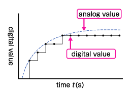
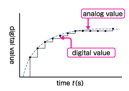
This is a graph of analog value over time. As can be seen, when the fluctuation of the leftmost analog value is converted to a digital value, the graph at the right end, high resolution, produces a value closer to the analog value than the graph in the middle, low resolution. Therefore, the higher the resolution, the more accurate measurement results can be displayed.
Also, the time on the horizontal axis is the same. By outputting data in as short a time as possible, time changes can be measured in detail. In this case, the processing speed of the computer and A/D conversion board has been improved, so it is possible to measure in a much shorter time compared to 10 years ago and 20 years ago.
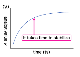
High-speed measurement is not always synonymous with high accuracy. Simply increasing the sampling rate can introduce noise, especially when measuring small signals. This is analogous to photography in low light: a faster shutter speed results in a grainy (noisy) image, while a longer exposure accumulates more light for a clearer picture.
In electronic measurement, extending the integration time or averaging multiple samples can significantly reduce random noise and improve measurement stability. For instance, a fluctuation of 1 count is significant in a 10-count sample but negligible in a 10,000-count sample. Therefore, selecting the appropriate integration time and sampling rate is essential based on the target application--whether measuring static voltage, transient switching timing, or environmental temperature.
Therefore, it is necessary to carefully consider the measurement timing and the integration (accumulation) time used for measurement. It is important to consider what design is required and what pattern of measurement may be possible when measuring voltage and current values, measuring switching timing, measuring resistance, measuring the operating environment temperature, etc.
Recommended products
Matsusada Precision's high-performance power supplies

Reference (Japanese site)
- Japanese source page 「デジタル計測と分解能 ~IoTの基礎(1)~」
(https://www.matsusada.co.jp/column/column-iot1-digital-resolution.html) - トランジスタ技術SPECIAL No.53 Winter
- 計測と制御 第41巻第1号 2002年1月号「歴史が選んだ計測器」
(https://www.jstage.jst.go.jp/article/sicejl1962/41/1/41_1_53/_pdf) - 東北大学大学院情報科学研究科 鏡慎吾 「イメージセンサの基礎」
http://www.ic.is.tohoku.ac.jp/~swk/lecture/ic2005/kagami_ic20050419.pdf (non-HTTPS address) - シーケンス制御講座「アナログ変換」
(https://news.aperza.jp/シーケンス制御講座「アナログ変換」/)